Configuration integral (statistical mechanics)
From VQWiki Public
by Loc Vu-Quoc
The classical configuration integral,
sometimes referred to as
the configurational partition function[1],
for a system with
 particles
is defined as follows:
particles
is defined as follows:
![\displaystyle
Z_N
:=
\int\limits_V
\exp
\left[
- \beta U (x_1 , \cdots , x_N)
\right]
d^3 x_1 \cdots d^3 x_N](/web/20120428193950im_/http://clesm.mae.ufl.edu/wiki.pub/images/math/c/8/9/c890ad5b350210cddf75bdac01aa2f3b.png)
(1)
where
 is
the volume enclosing the
particles,
is
the volume enclosing the
particles,
 a constant defined as

(2)
with
 being the
Boltzmann constant,
being the
Boltzmann constant,
 the
thermodynamic temperature[2]
the
thermodynamic temperature[2]
 the potential energy of interparticle forces,
 the positions in the 3-D space
 of the
particles, with
of the
particles, with
 and
and
 the
the
 coordinate of the
 particle,
and
particle,
and
 an infinitesimal volume.
An example for the potential energy
is the
Lennard-Jones potential.
an infinitesimal volume.
An example for the potential energy
is the
Lennard-Jones potential.
By setting
 , we have
 .
Since both
and
.
Since both
and
 have the dimension of energy, the integrand in
Eq.(1) is dimensionless,
and thus
the configuration integral
have the dimension of energy, the integrand in
Eq.(1) is dimensionless,
and thus
the configuration integral
 has the dimension of
 .
For this reason, some authors use the non-dimensionalized
configuration integral obtained by dividing Eq.(1) by
; see also
Allen & Tildesley (1989)[3],
p.41;
McComb (2004)[4],
p.95.
.
For this reason, some authors use the non-dimensionalized
configuration integral obtained by dividing Eq.(1) by
; see also
Allen & Tildesley (1989)[3],
p.41;
McComb (2004)[4],
p.95.
We begin to motivate by providing important applications of the configuration integral, then proceed to give a detailed derivation of Eq.(1) in a self-contained manner that does not require too many prerequisites[5].
|
|
Motivation
Disease research and drug design

By way of motivation for learning about the configuration integral, we consider an important application of the configuration integral in the development of computational models for the ligand-receptor binding affinities, the study of which constitutes a most important problem in computational biochemistry; Swanson et al. (2004)[6], see also Receptor (biochemistry). Research in the prediction of binding affinities has been a continuing effort for more than half a century.
The Human Immunodeficiency Virus (HIV) that could induce AIDS (Acquired Immune Deficiency Syndrome) has wreaked havoc in several human communities in the world. An HIV virus, such as HIV-1, destroys a human cell by first entering the cell through the cell membrane. To this end, the HIV-1 virus would have its gp120 envelope glycoprotein bind first to the CR4 glycoprotein receptor in the cell membrane, then second to a chemokine receptor family (CXCR4 or CCR5) to initiate its entry into the cell; see the highly informative articles HIV, HIV structure and genome, and the references [7] [8]. A research program has been underway at NIH to develop HIV vaccine (particularly the so-called gp120 vaccines) by trying to understand, through atomistic simulations, a mechanism of how HIV virus evade antibody proteins that would block its binding to the chemokine receptor, thus preventing it from entering the cell[9]. Fig.1 shows an atomistic model of a ligand-receptor-ligand binding involving the HIV-1 virus gp120 envelope glycoprotein (ligand), the CR4 glycoprotein (receptor), and the b12 antibody protein (ligand).
In a ligand-receptor binding, a ligand is in general any molecule that binds to another molecule; the receiving molecule is called a receptor, which is a protein on the cell membrane or within the cell cytoplasm. Such binding can be represented by the chemical reaction describing noncovalent molecular association:

(3)
where
 represents the protein (receptor),
B the ligand molecule,
and
represents the protein (receptor),
B the ligand molecule,
and
 the bound ligand-receptor.
A goal is to compute the change in the Gibbs energy[10] for the above reaction[11], which is given in terms of the configuration integrals as follows [12]

(4)
where the
 quantities are the configuration integrals.
For example, the configuration integral for protein
is
quantities are the configuration integrals.
For example, the configuration integral for protein
is
![\displaystyle
Z_{N,A}
=
\int
\exp
\left[
- \beta U(r_A , r_S)
\right]
d r_A d r_S](/web/20120428193950im_/http://clesm.mae.ufl.edu/wiki.pub/images/math/e/a/2/ea249b2a74fdbf57c50308d432773687.png)
(5)
The details on the other quantities are irrelevant for the present article, whose aim is to explain the origin of the configuration integral in statistical mechanics. Readers interested in understanding Eq.(4) are referred to Gilson et al. (1997)[12] for a detailed derivation. A recent review of the ligand-receptor affinity calculation is given by Gilson & Zhou (2007)[13].
Classical partition function (sum-over-states)
In classical (no quantum effect)
statistical mechanics,
the configuration integral
and
the partition function
 are fundamental in the study of
monoatomic, imperfect, classical gases and liquids.
Once these functions are known, the
thermodynamic properties
can be calculated.
For such a system with identical
particles,
the classical
partition function[14]
is obtained
by multiplying
the configuration integral
with a "momentum integral",
i.e., an integral over the momentum space,
whereas the configuration integral is an integral over
the configuration space, with the product of the configuration space
by the momentum space being the phase space[15].
In other words,
in parallel with the Hamiltonian being
the sum of the kinetic energy and the potential energy,
the partition function can be decomposed into a product of
the "momentum integral" (related to the kinetic energy)
and the configuration integral (related to the potential energy).
On the other hand, unlike the configuration integral,
which is in general difficult to integrate (because
of the complex nature of the potential energy),
this "momentum integral" can be easily integrated exactly
(because of the simple nature of the kinetic energy)
to yield a function of
the number
of particles
and the thermodynamic
temperature[2]
:
are fundamental in the study of
monoatomic, imperfect, classical gases and liquids.
Once these functions are known, the
thermodynamic properties
can be calculated.
For such a system with identical
particles,
the classical
partition function[14]
is obtained
by multiplying
the configuration integral
with a "momentum integral",
i.e., an integral over the momentum space,
whereas the configuration integral is an integral over
the configuration space, with the product of the configuration space
by the momentum space being the phase space[15].
In other words,
in parallel with the Hamiltonian being
the sum of the kinetic energy and the potential energy,
the partition function can be decomposed into a product of
the "momentum integral" (related to the kinetic energy)
and the configuration integral (related to the potential energy).
On the other hand, unlike the configuration integral,
which is in general difficult to integrate (because
of the complex nature of the potential energy),
this "momentum integral" can be easily integrated exactly
(because of the simple nature of the kinetic energy)
to yield a function of
the number
of particles
and the thermodynamic
temperature[2]
:

(6)
where
the coefficient
 is defined as

Case 
Distinguishable particles 
Indistinguishable particles
(7)
and
the
thermal de Broglie wavelength
 defined as
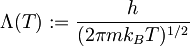
(8)
where
 is the
Planck constant.
See
further reading on .
is the
Planck constant.
See
further reading on .
It is sometimes mistaken to think of the configuration integral as
the same as the partition function,
modulo a multiplicative "constant".
First, as seen in Eq.(6), the multiplicative factor of
to obtain
is not a constant, but a function of
and
,
and is the result of integrating exactly
the "momentum integral".
Second, there are applications in which the configuration integral
plays an important role, with no direct role for the
"momentum integral", and therefore the partition function,
such as the example of assessing the
ligand-receptor binding affinity
mentioned above.
The abstract terminology "partition function" is also known more concretely and unassumingly as the "sum-over-states", which conveys a clear and direct meaning of this function, as shown in Eq.(33); see, e.g., Kirkwood (1933)[16]. Even though the name "partition function" (as used in statistical mechanics) is likely to first appear in 1922[17], in his classic book, Tolman (1938, 1979)[18], p.532, chose to use the name "sum-over-states", in agreement with what Planck (1932) used in German as "Zustandsumme" [19] [20] [21]. Other authors used the compromising, hybrid name "partition sum", e.g., Callen (1985), p.351[22]. Khinchin (1949)[23], p.76, used the name "generating function" for the partition function[24].
For the particular case where there is no potential, i.e.,
, such as in the case of
independent particles, the partition function
takes a
simple form.
As mentioned in the introduction,
the configuration integral
can be non-dimensionalized by dividing by
, with the non-dimensionalized version
denoted by
 . Then, the partition function
can be written as the product of
the partition function
. Then, the partition function
can be written as the product of
the partition function
 of ideal gas (i.e., when the potential
is zero)
by
the non-dimensionalized configuration integral
.
Thus, the configuration integral
can be thought of as a correction factor for
to obtain the partition function
for the case where the potential is non-zero.
of ideal gas (i.e., when the potential
is zero)
by
the non-dimensionalized configuration integral
.
Thus, the configuration integral
can be thought of as a correction factor for
to obtain the partition function
for the case where the potential is non-zero.
The power and elegance of statistical mechanics reside in its
application to predict accurately the thermodynamics properties
compared to experiments.
The knowledge of the partition function (and the corresponding
configuration integral) of a system is important since it allows for
the
calculation of thermodynamic properties.
For instance, a most important relation—sometimes referred
to as a fundamental relation; see Callen (1985), p.352[22]—connecting
statistical mechanics to
thermodynamics is the relationship between
the
Helmholtz energy[10]
and the partition function
 ;
McQuarrie (2000)[25], p.45:
;
McQuarrie (2000)[25], p.45:
![\displaystyle
A (T,V,N) = - k_B T \log Q (T,V,N)
\Longleftrightarrow
Q
=
\exp [- A / (k_B T)]
=
\exp (-\beta A)](/web/20120428193950im_/http://clesm.mae.ufl.edu/wiki.pub/images/math/5/a/9/5a92c4ef80ccffe290c12113a1f5989a.png)
(9)
with
 as defined in Eq.(2).
Some authors such as Callen (1985)
use the notation
as defined in Eq.(2).
Some authors such as Callen (1985)
use the notation
 ,
instead of the more historical and customary
notation
,
for the Helmholtz (free) energy[10][26].
Eq.(9)2
plays an important role in the
Jarzynski equality,
also known as a non-equilibrium work relation;
see the seminal paper by
Jarzynski (1997)[27], where the notation
was used for the
Helmholtz energy[10][26].
,
instead of the more historical and customary
notation
,
for the Helmholtz (free) energy[10][26].
Eq.(9)2
plays an important role in the
Jarzynski equality,
also known as a non-equilibrium work relation;
see the seminal paper by
Jarzynski (1997)[27], where the notation
was used for the
Helmholtz energy[10][26].
Physics of fluid turbulence
The configuration integral in particular, and statistical mechanics in general, have been used in the modelling of fluid turbulence; see, e.g., McComb (1992)[28], p.193.
Calculating the configuration integral
The dependence of the interparticle forces on the distance between the
particles makes the evaluation of the configuration integral
in Eq.(1)
"extremely difficult";
such evaluation has been driving much of the research in
classical statistical mechanics;
McQuarrie (2000)[25], p.116.
There are two methods to calculate a configuration integral: (i) approximate methods, and (ii) direct numerical integration.
For dilute gases in which the potential is of the usual type,
an expansion of the integrand of Eq.(1) in the powers of
![\displaystyle [\exp(-\beta U) - 1]](/web/20120428193950im_/http://clesm.mae.ufl.edu/wiki.pub/images/math/6/c/c/6cc8b90bda04c6cba20ab8a9abde7fc8.png) provides a systematic method to approximately calculate the
configuration integral
.
This method
is known as cluster expansion,
which
Maria Göppert-Mayer
contributed to develop;
See
Assael et al. (1996)[29],
p.49;
Huang (1987), p.213[30].
provides a systematic method to approximately calculate the
configuration integral
.
This method
is known as cluster expansion,
which
Maria Göppert-Mayer
contributed to develop;
See
Assael et al. (1996)[29],
p.49;
Huang (1987), p.213[30].
The direct numerical evaluation of the configuration integral is discussed in Tafipolsky et al. (2005)[31].
As mentioned,
we will build up below the fundamental
concepts that lead to the expression for
the classical
partition function
in Eq.(6)
and
the classical configuration integral
in Eq.(1),
so that all terms in
these expressions are explained, without requiring
too many prerequisites.
Systems with independent particles
Equilibrium, independent particles
According to the orthodox thermodynamic theory,
a thermodynamic system is in equilibrium if its thermodynamic state,
which is
a set of values for its thermodynamic parameters
(i.e., macroscopic parameters such as pressure
 , volume
, temperature
, magnetic field
, volume
, temperature
, magnetic field
 , etc.),
remains constant in time;
see, e.g.,
Sklar (1993)[32],
p.22,
Huang (1987)[30], p.3.
A quantitative condition of equilibrium can be described as the partial
time derivative of the distribution density being zero, i.e.,
the distribution density is time-independent at any fixed point in
the phase space; this condition is related to the
Liouville theorem;
see, e.g., Tolman (1979), p.55.
, etc.),
remains constant in time;
see, e.g.,
Sklar (1993)[32],
p.22,
Huang (1987)[30], p.3.
A quantitative condition of equilibrium can be described as the partial
time derivative of the distribution density being zero, i.e.,
the distribution density is time-independent at any fixed point in
the phase space; this condition is related to the
Liouville theorem;
see, e.g., Tolman (1979), p.55.
A more advanced and abstract concept of equilibrium came from the development of the kinetic theory, the criticisms of this theory, and the response of the proponents of the kinetic theory to these criticisms. In this concept, equilibrium does not characterize any single macroscopic state of the system, but rather a class of macrostates with each macrostate having its own probability; this approach is known as a reduction of thermodynamics to statistical mechanics; Sklar (1993)[32], p.23. This theory in turn had been a subject of criticism as to how the probabilistic assumptions, thought to be derived from the micro-constituents (atomic structure), were introduced into the theory.
Another line of reduction of thermodynamics to statistical mechanics allowed for the modeling of fluctuations around an equilibrium state. The work on this theory can be traced back to Einstein. Here, unlike the orthodox thermodynamic theory, an isolated system in contact with a heat bath at a constant temperature would have a range of internal temperatures and internal energy contents, centered on the temperature and internal energy of macroscopic equilibrium as predicted in the orthodox thermodynamic theory. This work was described by Sklar (1993) as of "surpassing elegance".
Deeper foundational issues on the definition of equilibrium will become more abstract and complex. The interested reader is referred to Sklar (1993)[32], Chapter 2, Section 2.II.6, pp.44-48, kinetic theory, ensemble approach and ergodic theory; Section 2.III, pp.48-59, Gibbs' statistical mechanics; Section 2.IV, pp.59-71, criticism of Gibbs' approach by the Ehrenfests. Chapter 5, p.156, detail discussion of equilibrium theory. A shorter version can be found in Sklar (2004)[33].
Basically, the historical development of statistical mechanics is rather entangled, with many branches, foundational issues, and problems to explore and resolve. Such confusion manifests itself through the existence of a dozen or so schools of thoughts in statistical mechanics with conflicting approaches: Ergodic theory, coarse-graining (Markovianism), interventionism, BBGKY hierarchy [34] [32], Jaynes, the Brussels school with De Donder[35], Prigogine, etc.; see Uffink (2004)[36], [37]. Disagreements among some of these schools can be found in further reading. The confusion came from the works of Boltzmann himself, who pursued different lines of thoughts; he would often abandon a line of thoughts, only to come back to it several years later[36].
Here, we only need to use the orthodox definition of equilibrium for the purpose of explaining the origin of the configuration integral, and follow Hill (1960, 1986)[38] and McQuarrie (2000)[25].
The particles in a system are considered as independent when there is a weak interaction among them that only involves collision between the particles or between a particle and the surrounding wall. There is no (or negligeable) interparticle forces. Without interaction among the particles, the system cannot reach an equilibrium, Hill (1986), p.59.
One way to think of this problem is by considering an unconfined space, with no walls, in which the particles can move without colliding against each other. Assuming no external forces, such as gravitational forces, the particles continue to move on a straight line with constant velocity. Macroscopically, there cannot be an equilibrium state. In other words, to achieve a macroscopic equilibrium, it is necessary that there be at least the kind of "weak interaction" mentioned above.
Admittedly, the above concept of equilibrium and independence among the particles is somewhat intuitive and hand-waving. It would be desirable to put the above concept on a more solid theoretical footing.
Independent particles
For systems with independent particles, there are two cases to consider: (1) Identical and distinguishable particles, and (2) Indistinguishable (or quantum-mechanically identical) particles.
It should be noted that in case (1), even though the particles are distinguishable, e.g., by their positions, they are identical in all other properties. An example would be the model of a monoatomic crystal, in which each atom is attached to a particular lattice site, and cannot jump to another lattice site. While these atoms are identical to each other, they are distinguishable by their locations in the crystal lattice; see Hill (1986), p.61.
Case (2) is related to a quantum-mechanical system in which identical particles are indistinguishable.
There may be a confusion in the use of the adjective "identical" in both cases. To distinguish the above two different types of "identical" particles, in case (1), we say the particles are identical (but distinguishable), whereas in case (2), we say that the particles are quantum-mechanically identical, which means the same as being indistinguishable. For a philosophical discussion, see French (2006) [39].
Distinguishable and identical particles
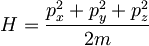
The classical Hamiltonian
 of a particle is given by

(21)
where
 represents the position vector of the particle,
 its linear momentum,
 its kinetic energy,
its potential energy,
its kinetic energy,
its potential energy,
 its mass,
and
its mass,
and
 its velocity.
For a system of
independent particles, the Hamiltonian is
![\displaystyle
H
=
\sum_{i=1}^{N} H_i
=
\sum_{i=1}^{N}
\left[
\frac
{p_i^2}
{2 m_i}
+
U (x_i)
\right]](/web/20120428193950im_/http://clesm.mae.ufl.edu/wiki.pub/images/math/7/7/e/77e8fb06a5b05e63c2a0cd6990233a50.png)
(22)
Even though it is possible to explain the configuration integral strictly within the framework of classical statistical mechanics, it is more general and simpler to develop the formulation within the framework of quantum statistical mechanics, which includes the classical statistical mechanics as a particular case; Hill (1986), p.2.
For a single particle in 1-D,
the system is quantized
(see
canonical quantization
)
by replacing the
classical Hamiltonian
by the Hamiltonian operator
 in which
the momentum is replace by the momentum operator
in which
the momentum is replace by the momentum operator

(23)
with
 being the unit imaginary number,
so that
being the unit imaginary number,
so that

(24)
In 3-D, the Hamiltonian operator
takes the form:

(25)
where
 is the divergence operator

(26)
The Schrödinger equation then takes the form

(27a)
where
 is a wave function (an eigenfunction), and
 the corresponding energy (eigenvalue).
The energy and the corresponding wave function constitute an
eigenpair, called a quantum state; there are infinitely many
such eigenpairs
the corresponding energy (eigenvalue).
The energy and the corresponding wave function constitute an
eigenpair, called a quantum state; there are infinitely many
such eigenpairs

(27b)
There will be multiple eigenvalues; the multiplicity of an eigenvalue
is called a degeneracy number denoted by
 .
.
The eigenpairs can be grouped by
energy level
 ,
i.e., by
the numerical values of the energy
(eigenvalue) ;
each energy level
thus has
,
i.e., by
the numerical values of the energy
(eigenvalue) ;
each energy level
thus has
 quantum states (eigenpairs) with the same energy value
 ,
but with different wave functions
,
but with different wave functions
 ,
,
 .
The set of quantum states at energy level
is
.
The set of quantum states at energy level
is

For a system of
independent particles,
similar to Eq.(22),
the system Hamiltonian operator is the sum of
the Hamiltonian operator of individual particle:

(28)
We reserve the index
 to designate the particle number,
the index
to designate the particle number,
the index
 for the quantum state, i.e., the eigenpair number, and the index
for the energy level.
for the quantum state, i.e., the eigenpair number, and the index
for the energy level.
Consider the system wave function of the form

(29)
Then (cf. Hill (1986), p.60),

(30)
Thus, the energy of the system is the sum of the energies of individual particles:

(31)
Hidden in Eq.(31) is the sum over all possible quantum states for each
particle. Let
 represent the state index for particle
,
and
represent the state index for particle
,
and
 the energy corresponding to state
of particle
.
Then
the energy corresponding to state
of particle
.
Then

(32)
is the energy corresponding to the system state
identified by the n-tuple
 .
.
The partition function
(or sum-over-states)
of particle
is of the form

(33)
where the sum is over all quantum states.
Likewise, the partition function for a system of independent and distinguishable particles is (cf. Hill (1986), p.60)

(34)
In addition to being independent and distinguishable, if the particles are also identical, then

(35)
and

(36)
Indistinguishable particles
Quantum-mechanically
identical particles are
indistinguishable. Roughly speaking, each n-tuple
has
 identical permutations, and thus the partition function
in Eq.(36) should be divided by
, i.e.,
identical permutations, and thus the partition function
in Eq.(36) should be divided by
, i.e.,

(51)
The justification for Eq.(51) is actually more sophisticated.
Consider identical, indistinguishable particles, labeled
 for the convenience of making the argument.
Consider different quantum states labeled
for the convenience of making the argument.
Consider different quantum states labeled
 with
with
 .
By permutations,
in the partition function
.
By permutations,
in the partition function  in Eq.(36),
there are
identical
terms
of the
form
in Eq.(36),
there are
identical
terms
of the
form
![\displaystyle
\exp
\left[
- \beta
(
\varepsilon_{a, j_a}
+
\varepsilon_{b, j_b}
+
\varepsilon_{c, j_c}
+
\cdots
)
\right]](/web/20120428193950im_/http://clesm.mae.ufl.edu/wiki.pub/images/math/9/2/e/92eb0d84aa9c3738c1b2875f36688e66.png)
(52)
Only one term among the
should be counted in the partition function.
But there also terms such as
![\displaystyle
\exp
\left[
- \beta
(
\varepsilon_{a, {\color{Red}\underset{=}{j_a}}}
+
\varepsilon_{b, {\color{Red}\underset{=}{j_a}}}
+
\varepsilon_{c, j_c}
+
\cdots
)
\right]](/web/20120428193950im_/http://clesm.mae.ufl.edu/wiki.pub/images/math/9/3/a/93a63ccad2a9bf1bf34968ed6439db1c.png)
(53)
where the energy level of the first two particles are the same;
by permutations of the last
 particles,
there are
particles,
there are
 such terms.
There are many other similar terms in which a subset of
two or more
particles
have an identical energy level.
such terms.
There are many other similar terms in which a subset of
two or more
particles
have an identical energy level.
Terms like those in Eq.(53), with repeated energy levels, are allowed in the Bose-Einstein statistics for bosons, but not allowed in the Fermi-Dirac statistics for fermions.
But in the limiting case in which
each particle has a number of quantum
states
between the molecular ground state and the molecular ground
state plus, say,
 ,
much larger than the number of
particles
,
then the number of terms such as those in Eq.(52)
is much larger than the number of terms such as those in Eq.(53),
since there are many different quantum states to choose from;
see Hill (1986), p.63.
Hence, the partition function can be
approximated
by
,
much larger than the number of
particles
,
then the number of terms such as those in Eq.(52)
is much larger than the number of terms such as those in Eq.(53),
since there are many different quantum states to choose from;
see Hill (1986), p.63.
Hence, the partition function can be
approximated
by

(54)
Thus Eq.(51) should actually be thought of as an approximation, rather than exact equality.
The above limiting case for which Eq.(51) is valid is called the
classical statistics or
Boltzmann statistics
,
which is the limit of the Bose-Einstein statistics and the Fermi-Dirac
statistics as temperature increases
 .
.
Ideal monoatomic gases
There are
independent
and
indistinguishable (quantum-mechanically identical)
particles
in a cubic box of side length
 .
To compute the partition function
.
To compute the partition function
 of this system, we need to
know the energy
levels of a single
particle in a box,
which is
a classic problem.
of this system, we need to
know the energy
levels of a single
particle in a box,
which is
a classic problem.
Particle in a box
Energy levels
By solving the 3-D time-independent Schrödinger equation
for a particle of mass
,
in a box, as given

(61)
with zero potential inside the box, i.e.,
 ,
we obtain the following
energy levels
(eigenvalues)
,
we obtain the following
energy levels
(eigenvalues)

(62)
where
 are the
quantum numbers,
which take natural values in
are the
quantum numbers,
which take natural values in
 ,
i.e.,
,
i.e.,
 .
.
Condition for approximation of partition function
As mentioned above,
the number of
quantum states
 available between
the ground state and the ground state plus
should be much larger than the number of particles
for the approximation in Eq.(54) to be valid, i.e.,
available between
the ground state and the ground state plus
should be much larger than the number of particles
for the approximation in Eq.(54) to be valid, i.e.,

(63)
Thus if we can connect the number
of quantum states to a given maximum
energy level
 ,
then we can establish an energetic condition
for which the approximation in Eq.(54) is valid.
,
then we can establish an energetic condition
for which the approximation in Eq.(54) is valid.
Consider Eq.(62) and the 3-D space of quantum numbers
.
Each point of natural-number coordinates in this space corresponds
to a quantum state, which can be thought of as occupying a unit
cube with a unit volume in this space.
Because of the factor
 in Eq.(62),
let's consider
a sphere in the space of quantum numbers, centered at the origin,
and having a radius
in Eq.(62),
let's consider
a sphere in the space of quantum numbers, centered at the origin,
and having a radius
 such that

(64)
Setting
 , we
would have the expression of the radius
, we
would have the expression of the radius
 such that the quantum states
on the surface of that sphere would have the energy level
such that the quantum states
on the surface of that sphere would have the energy level

(65)

Since the quantum numbers are natural numbers
(strictly positive integers),
the quantum states lie in an octant (1/8th of the sphere).
Thus, the volume of an octant with radius
contains all quantum states with energy levels less than
, i.e.,
this volume is equal to
the number of quantum states
with energy less than
:

(66)
with
 being the volume of the cube of length
.
Fig.2 illustrates the quantum states
in the space of quantum numbers
being the volume of the cube of length
.
Fig.2 illustrates the quantum states
in the space of quantum numbers
 :
The circle with radius
corresponds to the energy level
;
the quantum states outside the band corresponding to the energy
levels
and
:
The circle with radius
corresponds to the energy level
;
the quantum states outside the band corresponding to the energy
levels
and
 are represented
small open circles; the quantum states inside that "energy band"
are the small solid circles; the number of small solid circles is the
degeneracy at energy level
;
cf. McQuarrie (2000), p.11, Hill (1986), p.75.
are represented
small open circles; the quantum states inside that "energy band"
are the small solid circles; the number of small solid circles is the
degeneracy at energy level
;
cf. McQuarrie (2000), p.11, Hill (1986), p.75.
Now, take
of the order of
, i.e.,

(67)
then the condition in Eq.(63) becomes

(68)
where
is the thermal de Broglie wavelength in Eq.(8).
The factor 1.33 can be dismissed from the inequality in Eq.(68),
which becomes

(69)
i.e., for the partition function
in Eq.(51)
to be a good approximation,
the average distance between the particles should be much greater
than the thermal de Broglie wavelength
;
otherwise, quantum effects will not be negligible.
It is seen that the condition in Eq.(69) led to the
approximation in Eq.(54), and is therefore
the sufficient condition for the validity of
the application of
the classical or Boltzmann statistics
as expressed in the partition function
in Eq.(51).[40]
Discrete energy, continuous energy
Here, there is a potential confusion due to the use of the notation
to designate the
degeneracy[41]
in both the discrete (quantum) energy case
and in the continuous energy case.
For the discrete-energy case,
the summation in the
partition function
for a single particle
can be written in two
ways (cf. Eq.(33)):
(1) In terms of the quantum states, and
(2) in terms of the energy levels.
The summation in terms of the energy
levels itself has been written in two ways:
(2a) With a summation index for the energy level; this summation
index (a discrete variable) takes values in the set of natural numbers
, e.g.,
 .
(2b) Without a summation index, but using the
notation for energy
to designate a discrete variable
that takes values in the set of distinct energy levels, i.e.,
.
(2b) Without a summation index, but using the
notation for energy
to designate a discrete variable
that takes values in the set of distinct energy levels, i.e.,
 , such that
 ,
i.e., each energy level
,
i.e., each energy level
 has a different value of energy; there is no value that is repeated.
The 3 ways of writing the summation
in the partition function
has a different value of energy; there is no value that is repeated.
The 3 ways of writing the summation
in the partition function
 (i.e., 1, 2a, 2b above)
for a single particle
are presented below
(i.e., 1, 2a, 2b above)
for a single particle
are presented below

(70)
For the continuous-energy case, some authors wrote the partition
function
as
[Hill (1986), p.77; McQuarrie (2000), p.82]

(*)
Here is the confusion: The quantity
 in Eq.(70) is the degeneracy at the energy level
, i.e.,
the number of quantum states at the same energy level
,
whereas the quantity
in Eq.(*) is not the degeneracy, but the number of quantum states
per unit energy at the energy level
.
McQuarrie (2000), p.82, called the factor
in Eq.(70) is the degeneracy at the energy level
, i.e.,
the number of quantum states at the same energy level
,
whereas the quantity
in Eq.(*) is not the degeneracy, but the number of quantum states
per unit energy at the energy level
.
McQuarrie (2000), p.82, called the factor
 in Eq.(*) the "effective degeneracy", which is not
immediately clear at first encounter.
The dimensions of these two
's
are different from each other
(one is number of quantum states, the other is
number of quantum states per unit energy).
Thus it is better to write Eq.(*) with a different notation,
say
in Eq.(*) the "effective degeneracy", which is not
immediately clear at first encounter.
The dimensions of these two
's
are different from each other
(one is number of quantum states, the other is
number of quantum states per unit energy).
Thus it is better to write Eq.(*) with a different notation,
say
 ,
for the number of quantum states per unit energy:
,
for the number of quantum states per unit energy:

(71)
The case of continuous energy has two useful applications: (1) approximate a densely populated spectrum of discrete quantum energy levels in the evaluation of the partition function (see the next few subsections), (2) use in classical statistical mechanics where the energy varies continously, as opposed to the discrete energy in quantum mechanics.
Approximate summation by integration
With the expression in Eq.(62) for the energy levels for a particle in a box, the partition function expression in Eq.(70) becomes

(72)
The summation in Eq.(72) can be approximated by an integration of
the type shown in Eq.(71) if the summand in Eq.(72) changes
essentially continuously
with increments of the indices
 .
Such is the case if
.
Such is the case if

(73)
with
defined in Eq.(2), and
 the increment in energy level due to an increment of the indices
.
Based on the expression of the energy level in Eq.(62),
consider a unit increment of the quantum numbers
from
the increment in energy level due to an increment of the indices
.
Based on the expression of the energy level in Eq.(62),
consider a unit increment of the quantum numbers
from
 to
to
 ,
the increment in the energy level is of order
,
the increment in the energy level is of order

Thus, using the expression for the thermal de Broglie wavelength
in Eq.(2), we have

(74)
With the restriction that the average distance between the particles much larger than the thermal de Broglie wavelength, as expressed in Eq.(69), so that the approximated partition function in Eq.(54) become accurate, we have

(75)
If
is of the order of the
Avogadro number,
then

(76)
which largely satisfies the condition
in Eq.(73)[42], so that the summation in the partition function
in Eq.(72) can be approximated by the integration as expressed
in Eq.(71).
Effective degeneracy, order of magnitude
Now that we have introduced the different notation
for the number of quantum states per unit energy as shown in Eq.(71),
the "effective degeneracy" can be written as

(81)
We note immediately that the effective degeneracy
 is not the same as the degeneracy
, hence the difference
in notation.
is not the same as the degeneracy
, hence the difference
in notation.
As illustrated in Fig.1,
the effective degeneracy
 is
the number of quantum states lying inside the band formed by
the circle with radius
corresponding to the energy level
and a (slightly) larger circle corresponding to the energy level
;
Hill (1986), p.77; McQuarrie (2000), p.11.
We have
is
the number of quantum states lying inside the band formed by
the circle with radius
corresponding to the energy level
and a (slightly) larger circle corresponding to the energy level
;
Hill (1986), p.77; McQuarrie (2000), p.11.
We have

(82)
To give an idea about the magnitude of the effective degeneracy,
consider the following numerical data with
 (in SI units)

- Temperature

- Mass


- Box length

- Increment of energy

If we just look at the order of magnitude, then


and thus
![\displaystyle
\omega(\varepsilon_0, d \varepsilon)
=
O
\left[
\left(
\frac
{10^{25}}
{(10^{-34})^2}
\right)^{3/2}
\cdot
10^{-3}
\cdot
(10^{-21})^{1/2}
\cdot
10^{-2}
\cdot
10^{-21}
\right]
=
O(10^{28})](/web/20120428193950im_/http://clesm.mae.ufl.edu/wiki.pub/images/math/3/a/f/3afd4fd9ea5b7487c2cf99cea58baabe.png)
which is a large number for a simple system like a particle in a
box at room temperature; cf. McQuarrie (2000), p.11.
The order of magnitude of
 ,
i.e., the number of quantum states per unit energy, is then
,
i.e., the number of quantum states per unit energy, is then

which is much larger than the effective degeneracy
.
Partition function, thermal de Broglie wavelength
Using Eq.(82),
the partition function
in Eq.(71) for a particle in a box
can now be evaluated as follows
(Hill (1986), p.77)

(91)
where
, defined in Eq.(8),
is called the thermal de Broglie wavelength.
In Eq.(91), we made use of the following integration result
of the
Gamma function:

(92)
Integrating by parts the Gamma function in Eq.(92)1, we obtain:

(93)
Next, by changing the variable
 , we obtain

(94)
using the integration result in Eq.(162), noting that the domain of integration here is half that in Eq.(162). For more details on the Gamma function, the readers are referred to Sebah & Gourdon (2002)[43].
The thermal de Broglie wavelength
has the dimension of length (of course):
In the numerator of
,
the
Planck constant
has the dimension of energy times time, i.e.,
force
times length
times time
.
In the denominator of
,
the term
has the dimension of energy, i.e., force
times length
,
or equivalently
mass
times velocity squared
 .
Thus, the denominator has the dimension of mass
times velocity
, or momentum.
The dimension of
is then
.
Thus, the denominator has the dimension of mass
times velocity
, or momentum.
The dimension of
is then
![\displaystyle
[\Lambda]
=
\frac
{[h]}
{[m] [v]}
=
\frac
{FLT}
{(F L^{-1} T^2) \cdot (L T^{-1})}
=
L](/web/20120428193950im_/http://clesm.mae.ufl.edu/wiki.pub/images/math/3/4/7/3477f4373bc52a4613f6ebc4cb16c51a.png)
(95)
See
further reading on .
N particles in a box, partition function
The partition function of a system with
independent,
identical,
indistinguishable
particles
can now be written as

(101)
It can be verified that
in the absence of a potential energy, i.e.,
(since the particles are independent; there
is no interparticle forces),
the configuration integral
,
and
the partition function
in Eq.(6) is reduced to
Eq.(101).
Helmholtz energy
From Eq.(9),
the
Helmholtz energy[10][26]
of this system can now be written as

by using the
Stirling approximation
for
 , i.e.,

and
 .
Thus,
.
Thus,
![\displaystyle
A
=
-
k_B T
N
\log
\left[
\frac
{V e}
{\Lambda^3 N}
\right]
=
-
k_B T
N
\log
\left[
\frac
{(2 \pi m k_B T)^{3/2} V e}
{h^3 N}
\right]](/web/20120428193950im_/http://clesm.mae.ufl.edu/wiki.pub/images/math/2/8/f/28f94e3702955a2e1fdfdd09ef0db35f.png)
(102)
which can be used to calculate the thermodynamic properties of the system; see Hill (1986), p.77.
Thermodynamic properties
"the average physicist is made a little uncomfortable by thermodynamics. He is suspicious of its ostensible generality, and he doesn't quite see how anybody has a right to expect to achieve that kind of generality. He finds much more congenial the approach of statistical mechanics, with its analysis reaching into the details of those microscopic processes which in their large aggregates constitute the subject matter of thermodynamics. He feels, rightly or wrongly, that by the methods of statistical mechanics and kinetic theory he has achieved a deeper insight." P.W. Bridgman, The nature of thermodynamics, 1941, p.3.
Once the expression for the
Helmholtz energy
 is available,
one can then obtain the expressions for the
thermodynamic properties
of the
canonical ensemble,
i.e.,
entropy
is available,
one can then obtain the expressions for the
thermodynamic properties
of the
canonical ensemble,
i.e.,
entropy
 ,
pressure
,
pressure
 ,
chemical potentials
,
chemical potentials
 .
In addition, since
.
In addition, since
 , we can also obtain
the expression for the total
internal energy
of the system.
, we can also obtain
the expression for the total
internal energy
of the system.
Recall that the independent variables of the internal energy
for the canonical ensemble
are
entropy
,
volume
,
and
the particle numbers
 for different components (or species);
we write
for different components (or species);
we write
 .
We have
(McQuarrie (2000), p.17)
.
We have
(McQuarrie (2000), p.17)

(111)
being the chemical potential for species
 .
.
With the Legendre transformation
-
(112)
we have

(113)
making
 the independent variables for the Helmholtz energy
.
From Eq.(113) and using Eq.(9), we have
(cf. Hill (1986), p.19)
the independent variables for the Helmholtz energy
.
From Eq.(113) and using Eq.(9), we have
(cf. Hill (1986), p.19)

(114)

(115)

(116)
Finally,
using Eq.(114) in Eq.(9),
we obtain the expression for
the total internal energy

(117)
with
defined in Eq.(2).
Now using the expression for the Helmholtz energy
in Eq.(102)
and Eqs.(114)-(117),
we obtain the following expressions for the thermodynamic properties
for
an
ideal monoatomic gas
(i.e., a system of
distinguishable, identical, and
independent particles):
![\displaystyle
S
=
-
\left.
\frac
{\partial A}
{\partial T}
\right|_{V,N_\alpha}
=
\frac
{\partial [bT \log (a T^{3/2})]}
{\partial T}
=
b \log (a T^{3/2})
+
b T \frac{3}{2} T^{-1}
=
b \log (a T^{3/2} e^{3/2})](/web/20120428193950im_/http://clesm.mae.ufl.edu/wiki.pub/images/math/a/b/c/abc2185c962d2690ae5f30ce014d0f51.png)
where
and
 are constants with respect to
;
see Eq.(102).
Thus, the entropy for ideal monoatomic gas takes the form
(cf. Hill (1986), p.79)
are constants with respect to
;
see Eq.(102).
Thus, the entropy for ideal monoatomic gas takes the form
(cf. Hill (1986), p.79)
![\displaystyle
S
=
k_B N
\log
\left[
\frac
{(2 \pi m k_B T)^{3/2} V e^{5/2}}
{h^3 N}
\right]](/web/20120428193950im_/http://clesm.mae.ufl.edu/wiki.pub/images/math/3/c/c/3cc36e97264bb1487f10d41c95ee27b9.png)
(118)
Similarly, the pressure takes the familiar form of the ideal gas law:

(119)
Chemical potential for the case with one species:
![\displaystyle
\mu
=
\left.
\frac
{\partial A}
{\partial N}
\right|_{T,V}
=
-
k_B T
\log
\left[
\frac
{(2 \pi m k_B T)^{3/2} V}
{h^3 N}
\right]
=
-
k_B T
\log
\left[
\frac
{(2 \pi m k_B T)^{3/2} k_B T}
{h^3 p}
\right]](/web/20120428193950im_/http://clesm.mae.ufl.edu/wiki.pub/images/math/2/b/1/2b1ef474f71c43e98533de6d767e6d52.png)
(120)
where Eq.(119) had been used in the last equation. Thus, (cf. Hill (1986), p.80)
![\displaystyle
\mu
=
\mu_0 (T)
+
k_B T \log p
, \ {\rm with} \
\mu_0 (T)
=
-
k_B T
\log
\left[
\frac
{(2 \pi m k_B T)^{3/2} k_B T}
{h^3}
\right]](/web/20120428193950im_/http://clesm.mae.ufl.edu/wiki.pub/images/math/6/2/7/62787b4aaf5a6633f3cdb4717b50c710.png)
(121)
The internal energy
of an ideal monoatomic gas
follows from the expression for
in Eq.(102) and Eq.(112), and the expression for
in Eq.(118)

(122)
which is purely the kinetic energy of the system,
without the potential energy, since there were no interparticle forces.
The amount of kinetic energy
per momentum
degree of freedom (dof)
of the system
is
 (there are
 momentum dofs)[44].
Of course, the same result shown in Eq.(122)
can be obtained
by differentiating
the partition function
using
Eq.(117)2
or
Eq.(117)3.
Eq.(119) for pressure
and Eq.(122) for internal energy
are called the "classical results"
since they can be derived from using only the
kinetic theory,
without a need for a quantum-mechanical setting.
Here, we recover the classical results starting from a
quantum-mechanical setting, which is reassuring, and therein lies
the beauty and power of statistical mechanics.
momentum dofs)[44].
Of course, the same result shown in Eq.(122)
can be obtained
by differentiating
the partition function
using
Eq.(117)2
or
Eq.(117)3.
Eq.(119) for pressure
and Eq.(122) for internal energy
are called the "classical results"
since they can be derived from using only the
kinetic theory,
without a need for a quantum-mechanical setting.
Here, we recover the classical results starting from a
quantum-mechanical setting, which is reassuring, and therein lies
the beauty and power of statistical mechanics.
In this section, we have connected statistical mechanics and thermodynamics; such connection, having a starting point in statistical mechanics, is often known in philosophy as a reduction of thermodynamics to statistical mechanics, leading to an alternative name statistical thermodynamics for the field; see Sklar (2004)[33].
Average continuous energy, equipartition
The internal energy in
Eq.(122) can be obtained by computing the
average energy
as follows.
From the partition function Eq.(70)1
for discrete energy of a
single particle in a box,
the probability that the particle is found in state
 is[24]

(123)
and the average energy of a single particle is (cf. Hill (1986), p.12)

(124)
For the continous energy case, we obtain from Eq.(71)
the probability for a single particle
to be within the energy band
![\displaystyle [\varepsilon , \varepsilon + d \varepsilon]](/web/20120428193950im_/http://clesm.mae.ufl.edu/wiki.pub/images/math/5/9/b/59b1ce1a67328ed64bffcde114960fb4.png) as
(Hill (1986), p.77)
as
(Hill (1986), p.77)

(125)
and the average energy of a single particle as

(126)
Next, using
Eq.(91), i.e.,
the expression for
,
in
Eq.(126),
we have the average energy of a single particle as
(after cancelling out the common factor)

(127)
where we have made use of
Eq.(92)3
and
Eq.(93)2.
For a system with
particles, we then obtain the same result as in Eq.(122),
based on
Eq.(31)
(system energy is the sum of particle energy).
The above result for the ideal gas law in Eq.(119) and for the internal energy in Eqs.(122) and (127) can also be obtained using the equipartition theorem (Tolman (1979), p.93).
Classical statistical mechanics, continuous energy
In the limit of large quantum numbers, quantum statistics would asymptotically approach classical statistics. As temperature increases, terms corresponding to larger quantum numbers provide more important contribution to the overall sum in the canonical ensemble partition function. All results obtained from classical statistics, which is often easier to use, would be some limits of quantum statistics. Classical statistics is a special case of quantum statistics. We follow Hill (1986), p.112, to develop classical statistics inductively from the quantum statistics results obtained above.
One-dimensional harmonic oscillator
Energy
Classical case (continuous energy)
The potential energy
in a
classical harmonic oscillator
(spring-mass system)
with linear force-displacement relationship
is a quadratic form in the coordinate

(131)
where
 is the spring stiffness coefficient
[45],
and
the displacement.
is the spring stiffness coefficient
[45],
and
the displacement.
From Eq.(21), the classical Hamiltonian is now written as

(132)
The
classical frequency
 of this simple oscillator takes the form
[46]
of this simple oscillator takes the form
[46]

(133)
Thus, the Hamiltonian can be written in terms of the frequency
as follows
(cf. Hill (1986), p.113)

(134)
The Hamiltonian
in Eq.(134) is the total internal energy of the system, and is
continuous in terms of the phase-space variables
 .
.
Quantum case (discrete energy)
The energy levels of a quantum harmonic oscillator, obtained by solving Eq.(27a), are discrete and non-degenerate

(141)
where
is the
Planck constant,
the classical frequency in Eq.(133),
 ,
and
,
and
 the
circular frequency.
the
circular frequency.
Partition function
We begin by considering the partition function for the quantum harmonic oscillator, with discrete energy levels and its limiting case, then "generalize" to the partition function for the classical harmonic oscillator with continuous energy. The limiting case of the quantum partition function will be use to determine the constant for the classical partition function.
Quantum case
Using Eq.(70)1, the quantum partition function can be written as
![\displaystyle
q
=
\sum_{n=0}^{\infty}
\exp (- \beta \varepsilon_n)
=
\exp
\left(
- \frac{h \nu}{2 k_B T}
\right)
\sum_{n=0}^{\infty}
\exp
\left(
- \frac{n h \nu}{k_B T}
\right)
=
\exp
\left(
- \frac{h \nu}{2 k_B T}
\right)
\sum_{n=0}^{\infty}
\left[
\exp
\left(
- \frac{h \nu}{k_B T}
\right)
\right]^n](/web/20120428193950im_/http://clesm.mae.ufl.edu/wiki.pub/images/math/6/c/e/6ce68b65118ab2b9df0f06c668d6a1c6.png)

(151)
As temperature rises, i.e.,
,
thus
 ; a development in
Taylor series
leads to an asymptotic function in term of
for the partition function
(cf. Hill (1986), p.89)
; a development in
Taylor series
leads to an asymptotic function in term of
for the partition function
(cf. Hill (1986), p.89)

(152)
The above asymptotic function will be used to fix the proportionality constant in the classical partition function for the case with continuous energy.
Another way of obtaining the asymptotic function in Eq.(152) is to
follow the same line of argument made further above to
approximate summation by integration.
Since
is very small,
 is nearly equal to 1, and thus
![\displaystyle [\exp(-u)]^n](/web/20120428193950im_/http://clesm.mae.ufl.edu/wiki.pub/images/math/0/4/1/041a7f99bbb49b469338d1ecd9fb436f.png) would be essentially continuous with
would be essentially continuous with
 , i.e.,
the increment
, i.e.,
the increment
![\displaystyle
[\exp(-u)]^{n+1}
-
[\exp(-u)]^{n}](/web/20120428193950im_/http://clesm.mae.ufl.edu/wiki.pub/images/math/5/5/5/555a7ee8702cda2735c1e3c4060ee627.png)
is very small. In this case, the summation in Eq.(151) can be approximated by an integration, i.e.,
![\displaystyle
q
\approx
\exp
\left(
- \frac{h \nu}{2 k_B T}
\right)
\int\limits_{n=0}^{\infty}
\left[
\exp
\left(
- \frac{h \nu}{k_B T}
\right)
\right]^n
d n
=
\exp
\left(
- \frac{h \nu}{2 k_B T}
\right)
\frac
{1}
{\log \exp (h \nu / k_B T)}
\rightarrow
\frac
{k_B T}
{h \nu}](/web/20120428193950im_/http://clesm.mae.ufl.edu/wiki.pub/images/math/1/4/3/143c6c206ca44b483a9f738821f1bcb0.png)
(153)
since
![\displaystyle
\int\limits_{n=0}^{\infty}
\left[
\exp
\left(
- \frac{h \nu}{k_B T}
\right)
\right]^n
d n
=
\int\limits_{n=0}^{n=\infty}
a^{-n}
d n
=
-
\int\limits_{y=1}^{y=0}
y
\frac
{d y}
{y \log a}
=
\frac
{1}
{\log a}](/web/20120428193950im_/http://clesm.mae.ufl.edu/wiki.pub/images/math/5/a/7/5a759816e263195444e081420f20861a.png)
with

Average quantum energy, failure of equipartition

First, using Eq.(70)1, we can rewrite Eq.(124) as follows

(156)
Compare
Eq.(156)3
to
Eq.(117)3.
Next, with the partition function for a quantum harmonic oscillator
given in Eq.(151)4,
using
Eq.(156)3,
we obtain the average energy for the quantum harmonic
oscillator as
(cf. Tolman (1979), p.379; McQuarrie (2000), p.121, p.132)
![\displaystyle
\langle
\varepsilon
\rangle
=
\frac
{h \nu}
{2}
\left[
\frac
{1 + \exp (- \beta h \nu)}
{1 - \exp (- \beta h \nu)}
\right]
\rightarrow
k_B T
\ {\rm as} \
T \rightarrow \infty](/web/20120428193950im_/http://clesm.mae.ufl.edu/wiki.pub/images/math/7/a/3/7a3bbea4ad1c7762ee7cae24fa36ca45.png)
(157)
with
the limit of
 as
being the result of
using the same method as in Eq.(152).
Thus we have equipartition of energy for high temperature
,
half from the kinetic energy and half from the potential energy
(cf. Eq.(127) for a particle in a 3-D box where there was
only kinetic energy, with zero potential energy).
At low temperature
,
there was no equipartition of energy, i.e.,
equipartition does not work at low temperature
due to quantum effects.
Fig.3 shows the quantum correction to equipartition at
low temperature for the quantum harmonic oscillator and for
the electromagnetic oscillator
(which is used to explain black-body radiation)[47].
as
being the result of
using the same method as in Eq.(152).
Thus we have equipartition of energy for high temperature
,
half from the kinetic energy and half from the potential energy
(cf. Eq.(127) for a particle in a 3-D box where there was
only kinetic energy, with zero potential energy).
At low temperature
,
there was no equipartition of energy, i.e.,
equipartition does not work at low temperature
due to quantum effects.
Fig.3 shows the quantum correction to equipartition at
low temperature for the quantum harmonic oscillator and for
the electromagnetic oscillator
(which is used to explain black-body radiation)[47].
Classical case, phase integral
A logical "generalization" of the quantum partition function for discrete energy levels in Eq.(151)1, i.e.,

is to replace the quantum summation with
an integral for continuous energy to obtain the classical
partition function
 .
But it is not that simple;
to make sure that the classical partition function
agrees with the quantum partition function in the limit when
, i.e.,
.
But it is not that simple;
to make sure that the classical partition function
agrees with the quantum partition function in the limit when
, i.e.,

in Eqs.(152)-(153),
we need to add a
proportionality constant
 in the expression for
:
in the expression for
:
![\displaystyle
q_{class}
=
c
\iint\limits_{-\infty}^{+\infty}
\exp[ - \beta H (x,p)]
dx
dp
=
c
\iint\limits_{-\infty}^{+\infty}
\exp
\left[
-
\beta
\left(
\frac
{p^2}
{2 m}
+
2 \pi^2 m \nu^2
x^2
\right)
\right]
dx
dp](/web/20120428193950im_/http://clesm.mae.ufl.edu/wiki.pub/images/math/0/3/c/03c8c46c16e81e659b6ac0bd72a9d8c2.png)
![\displaystyle
=
c
\left(
\int\limits_{-\infty}^{+\infty}
\exp
\left[
-
\beta
\frac
{p^2}
{2 m}
\right]
dp
\right)
\left(
\int\limits_{-\infty}^{+\infty}
\exp
\left[
-
\beta
2 \pi^2 m \nu^2
x^2
\right]
dx
\right)
=
c
\sqrt{
\frac
{\pi}
{\beta / 2m}
}
\sqrt{
\frac
{\pi}
{\beta 2 \pi^2 m \nu^2}
}](/web/20120428193950im_/http://clesm.mae.ufl.edu/wiki.pub/images/math/b/c/0/bc068f166c42f0987ac5aaefea1bf946.png)

(161)
where we made use of the integration results
![\displaystyle
\left(
\int\limits_{x=-\infty}^{x=+\infty}
\exp (-x^2)
dx
\right)^2
=
\left(
\int\limits_{x=-\infty}^{x=+\infty}
\exp (-x^2)
dx
\right)
\left(
\int\limits_{y=-\infty}^{y=+\infty}
\exp (-y^2)
dy
\right)
=
\iint\limits_{-\infty}^{+\infty}
\exp [-(x^2 + y^2)]
dx
dy](/web/20120428193950im_/http://clesm.mae.ufl.edu/wiki.pub/images/math/0/9/0/0908efb13df54f6a007a626daf570b7e.png)

(162)
and

(163)
Thus (cf. Hill (1986), p.113)
![\displaystyle
q_{class}
=
\frac
{1}
{h}
\iint\limits_{-\infty}^{+\infty}
\exp[ - \beta H (x,p)]
dx
dp](/web/20120428193950im_/http://clesm.mae.ufl.edu/wiki.pub/images/math/f/0/c/f0c86c87910a5f71c654c0f0d78a5bdf.png)
(164)
The integral in Eq.(164) is carried over the whole phase space is called the phase integral.
Particle in a box
Recall from Eq.(72) that the quantum partition function for a particle in a box takes the form
At sufficiently high temperature,
,
the condition in Eq.(73) is
satisfied, i.e.,

and the quantum partition function can be approximated by an integration, leading to the expression in Eq.(91), i.e.,

Consider the following "generalization" of Eq.(72) to the case with continuous energy

(171)
with the Hamiltonian (or energy) being simply the kinetic energy (the potential energy is zero)
(172)
and

(173)
Using the integration result in Eq.(163),
and the fact that the classical partition function
is the limiting case of the quantum partition function
as
,
we have

(174)
Thus,

(175)
Hence, for a particle in a box with 3 momentum dofs and 3 position dofs[44] (see Hill (1986), p.115):

(176)
System of indistinguishable particles
Zero potential energy (without interparticle forces)
In general, for a particle system in a box with
momentum dofs and with zero potential energy,
the Hamiltonian is
purely kinetic energy

(181)
and the classical partition function takes the form

(182)
For a system of
particles in 3-D space
,
we have
 ,
which represents both
momentum dofs and
position dofs[44].
Without a zero potential energy,
the integration can be carried out
to yield
,
which represents both
momentum dofs and
position dofs[44].
Without a zero potential energy,
the integration can be carried out
to yield

(183)
The above partition function is for distinguishable particles.
For indistinguishabe particles, a division by
yields the classical partition function

(184)
which is the same as in Eq.(101).

An interpretation for the division by
in Eq.(184) can be given as follows.
Consider the case with two particles moving in a 1-D space, with
a 2-D phase space.
The phase integral in Eq.(184) can be approximated
by a quadruple summation
![\displaystyle
\sum_{x_1 \in \mathcal X}
\sum_{p_1 \in \mathcal P}
\sum_{x_2 \in \mathcal X}
\sum_{p_2 \in \mathcal P}
\exp[-\beta H (x_1, p_1, x_2, p_2)]
(d \tau)^2](/web/20120428193950im_/http://clesm.mae.ufl.edu/wiki.pub/images/math/4/e/a/4eafdba026fae2ff2e57bd54754bc323.png)
(185a)
where

(185b)
is an infinitesimal area in the phase space, as represented by a
green square in Fig.4.
The sets
 and
and
 are sets of discrete values of the continuous variables
 and
and
 ,
for
,
for
 :
:

(186)
The phase-space coordinates of particle
are denoted by
 .
In the summation in Eq.(185a), there are two terms that correspond
respectively to
(i) particle 1 (red dot in Fig.4) at position
in phase space, i.e.,
.
In the summation in Eq.(185a), there are two terms that correspond
respectively to
(i) particle 1 (red dot in Fig.4) at position
in phase space, i.e.,
 ,
and particle 2 (blue dot in Fig.4) at position
in phase space, i.e.,
,
and particle 2 (blue dot in Fig.4) at position
in phase space, i.e.,
 ,
and
(ii) particle 2 (blue dot in Fig.4) at position
in phase space, i.e.,
,
and
(ii) particle 2 (blue dot in Fig.4) at position
in phase space, i.e.,
 ,
and particle 1 (red dot in Fig.4) at position
in phase space, i.e.,
,
and particle 1 (red dot in Fig.4) at position
in phase space, i.e.,
 .
In the case where the particles are indistinguishable, the above two
cases represent only a single quantum state, i.e.,
the summation in Eq.(185a) thus double counted the number of states,
and thus should be divided by
the number of particles, i.e.,
.
In the case where the particles are indistinguishable, the above two
cases represent only a single quantum state, i.e.,
the summation in Eq.(185a) thus double counted the number of states,
and thus should be divided by
the number of particles, i.e.,
 .
.
For a system with
indistinguishable particles,
each state is counted
times, and thus a division by
in Eq.(184)
(cf. Hill (1986), p.117).
The above argument to justify for the factor
 was attributed to Gibbs,
and resolved the
Gibbs paradox
when mixing identical gases; see, e.g., Huang (1987), p.141.
Kirkwood (1934)[16],
considered this Gibbs argument "somewhat arbitrary",
provided a quantum-mechanical approach
to obtain the factor
; see also Hill (1986), p.462.
On the other hand, Buchdahl (1974)[48]
provided a justification based on purely
classical statistical mechanics.
was attributed to Gibbs,
and resolved the
Gibbs paradox
when mixing identical gases; see, e.g., Huang (1987), p.141.
Kirkwood (1934)[16],
considered this Gibbs argument "somewhat arbitrary",
provided a quantum-mechanical approach
to obtain the factor
; see also Hill (1986), p.462.
On the other hand, Buchdahl (1974)[48]
provided a justification based on purely
classical statistical mechanics.
A classical partition function (e.g., Eq.(182))
with a correction factor
such as shown in Eq.(184)
is sometimes referred to as a
semiclassical partition function; see, e.g.,
Kirkwood (1934),
Reichl (1998), p.359.
In the literature, there was some confusion in the terminologies used:
The phase integral—which
Kirkwood (1933)[16]
referred to as the Gibbs phase integral, and which does not
have the factor
 —was
sometimes called the "classical partition function" by some authors,
see, e.g., Zwanzig (1957)[49].
On the other hand, some other authors, such as Hill (1986),
referred to
the phase integral with the factor
,
with or without the correction factor
,
as the "classical partition function".
—was
sometimes called the "classical partition function" by some authors,
see, e.g., Zwanzig (1957)[49].
On the other hand, some other authors, such as Hill (1986),
referred to
the phase integral with the factor
,
with or without the correction factor
,
as the "classical partition function".
Non-zero potential energy (with interparticle forces)
When the potential energy is non-zero, i.e., there are interparticle forces, which is the more interesting and general case, the Hamiltonian is written as

(201)
where
 is the momentum of particle
along the
th
coordinate direction,
for
is the momentum of particle
along the
th
coordinate direction,
for
 and
and
 ,
the potential energy,
and
,
the potential energy,
and
 the position of particle
in 3-D space.
In this case, the classical partition function
in
Eq.(184)1
becomes
Eq.(6), after integrating out the kinetic energy part
(first term in Eq.(201)), i.e.,
the position of particle
in 3-D space.
In this case, the classical partition function
in
Eq.(184)1
becomes
Eq.(6), after integrating out the kinetic energy part
(first term in Eq.(201)), i.e.,

(6)
When there the potential function
,
we obtain
,
thus recovering
Eq.(184)2;
see Hill (1986), p.118.
Further reading
- Thermal de Broglie wavelength
- Boltzmann's Work in Statistical Physics, The Stanford Encyclopedia of Philosophy, Edward N. Zalta (ed.), First published Wed 17 Nov, 2004.
- Brussels or Brussels-Austin school in statistical mechanics
- Google search with keywords "brussels school statistical mechanics"
- Some Philosophical Influences on Ilya Prigogine's Statistical Mechanics
- Bishop, R.C., Brussels-Austin Nonequilibrium Statistical Mechanics in the Early Years: Similarity Transformations between Deterministic Probabilistic Descriptions, arXiv:physics/0304018v3, [physics.class-ph], 7 Apr 2003.
- Shalizi, C., Ilya Prigogine, Notebooks, 20 Aug 2007.
- Entropy in statistical mechanics, Chap.11, dissertation, University of Utretch, Netherlands.
- Disagreements with the Brussels-Austin school
- Bricmont, J., Science of Chaos or Chaos in Science?, arXiv:chao-dyn/9603009v1, Mar 1996.
- Dr. Prigogine's dissipative structure theory and some critical comments on this theory
Notes and references
- ↑ See, e.g., G.H. Wannier, Statistical Physics, Dover Publications, New York, 1987 (p.244, Read from Google Book); K. Lucas, Molecular Models for Fluids, Cambridge University Press, 2007 (p.270, Read from Google Book).
- ↑ 2.0 2.1 Some wiki pages for temperature: Wikipedia Sklogwiki (where the article has not been completed, but the reference to journal articles are quite up-to-date). Jones, E.R., Fahrenheit and Celsius, a history, The Physics Teacher, Nov. 1980, Vol.18, No.8, pp.594-595. PBS NOVA program Absolute Zero, aired in Jan 2008, or watch this program online. C. Shiller, Motion Mountain, (encyclopedic, unusual, free, online physics textbook), 21st edition, Dec 2007, Part I, Section on Temperature, pp.259-280.
- ↑ Allen, M.P., and Tildesley, D.J., Computer Simulation of Liquids, Oxford University Press, 1989. Read from Google Book.
- ↑ McComb, W.D., Renormalization Methods: A Guide for Beginners, Oxford University Press, 2004. Read from Google Book.
- ↑ The intention here is to make the article more useful for learning and research, rather than simply providing a list of formulas with superficial explanation. For this matter, see several useful articles in mathematics, e.g., Calculus of variations, etc. or even the classical mechanics article classical harmonic oscillator, which is closer to the present article.
- ↑ J. M. J. Swanson, R. H. Henchman, and J. A. McCammon, Revisiting Free Energy Calculations: A Theoretical Connection to MM/PBSA and Direct Calculation of the Association Free Energy, Biophys J. 2004 January; 86(1): 67–74.
- ↑ Kwong, P., et al. HIV-1 evades antibody-mediated neutralization through conformational masking of receptor-binding sites, Nature 420, 678-682 (12 December 2002).
- ↑ Kwong, P., et al. Structure of an HIV gp120 envelope glycoprotein in complex with the CD4 receptor and a neutralizing human antibody, Nature 393, 648-659 (18 June 1998)
- ↑ Peter D. Kwong, Ph.D., Vaccine Research Center, Structural Biology Laboratory, National Institute of Allergy and Infectious Diseases, National Institute of Health, Description of Research Program, 2007.
- ↑ 10.0 10.1 10.2 10.3 10.4
The
Gibbs energy
is customarily known as the
"Gibbs free energy",
and
the
Helmholtz energy
the
"Helmholtz free energy".
The name
"free energy"
was originally used by
Gibbs in 1876-1878,
and by
Lewis and Randall,
Thermodynamics and the Free Energy of Chemical Substances,
McGraw-Hill,
1923;
see the
Glossary of coined terms
in
J. Andraos'
Named Things in Chemistry & Physics.
The
IUPAC
recommends to use either
energy (more precise) or function (vague),
instead of "free energy".
Some comments in the literature related to the use
of "free energy":
 "A ... worst situation exists with the Gibbs and the Helmholtz
functions [energy]. The misnomer free energy
(which, by the way, is not energy but is freely misused) is employed by
American chemists to designate the Gibbs function, but by Europeans to
designate the Helmholtz function. To make matter worse, both groups
insist on using the same symbol
for the two different functions,"
p.350 in
M.W. Zemansky,
Fashions in Thermodynamics,
Am. J. Phys., Vol.25, No.6, pp.349-351, Sep 1957.
Of course, the Gibbs energy and the Helmholtz energy are different
kinds of energy. An example of an American physicist who associated
"free energy" to the "Helmholtz free energy"
is Huang (1987), p.22 and Index p.489.
"IUPAC banished the ambiguous term “free energy”
decades ago,"
p.754 in
R. Battino,
"Mysteries" of the First and Second Laws of Thermodynamics,
J. Chem. Edu., Vol.84, No.5, pp.753-755, May 2007.
The ambiguity of the name
"free energy"
can be seen in
the Interactive Link Maps
that show the many connections of other concepts to the
"free energy"
(which in the past was used for both
the Gibbs energy and the Helmholtz energy)
in the
Gold Book,
the IUPAC Compendium of Chemical Terminology.
The above two comments spanned exactly half a century, railing against
the use of "free energy", but without a complete success as the
terminology has been ingrained in many who grew up with it; see, e.g.,
Bevan Ott & Boerio-Goates (2000), p.xvi.
It is therefore important to know both
the currently recommended and the past usage
of different terminologies
so to read the classic (or even modern) works.
Here, we adhere to the IUPAC recommendations—and
I went "free" hunting in this article.
"A ... worst situation exists with the Gibbs and the Helmholtz
functions [energy]. The misnomer free energy
(which, by the way, is not energy but is freely misused) is employed by
American chemists to designate the Gibbs function, but by Europeans to
designate the Helmholtz function. To make matter worse, both groups
insist on using the same symbol
for the two different functions,"
p.350 in
M.W. Zemansky,
Fashions in Thermodynamics,
Am. J. Phys., Vol.25, No.6, pp.349-351, Sep 1957.
Of course, the Gibbs energy and the Helmholtz energy are different
kinds of energy. An example of an American physicist who associated
"free energy" to the "Helmholtz free energy"
is Huang (1987), p.22 and Index p.489.
"IUPAC banished the ambiguous term “free energy”
decades ago,"
p.754 in
R. Battino,
"Mysteries" of the First and Second Laws of Thermodynamics,
J. Chem. Edu., Vol.84, No.5, pp.753-755, May 2007.
The ambiguity of the name
"free energy"
can be seen in
the Interactive Link Maps
that show the many connections of other concepts to the
"free energy"
(which in the past was used for both
the Gibbs energy and the Helmholtz energy)
in the
Gold Book,
the IUPAC Compendium of Chemical Terminology.
The above two comments spanned exactly half a century, railing against
the use of "free energy", but without a complete success as the
terminology has been ingrained in many who grew up with it; see, e.g.,
Bevan Ott & Boerio-Goates (2000), p.xvi.
It is therefore important to know both
the currently recommended and the past usage
of different terminologies
so to read the classic (or even modern) works.
Here, we adhere to the IUPAC recommendations—and
I went "free" hunting in this article.
- ↑ After the kinetic contributions of each species have cancelled.
- ↑ 12.0 12.1 M. K. Gilson, J. A. Given, B. L. Bush and J. A. McCammon, The statistical-thermodynamic basis for computation of binding affinities: A critical review. Biophysical Journal 72: 1047-1069 (1997).
- ↑ M. K. Gilson and H.-X. Zhou, Calculation of Protein-Ligand Binding Affinities, Annual Review of Biophysics and Biomolecular Structure Vol. 36: 21-42 (Volume publication date June 2007).
- ↑ Some wiki pages on partition function: Sklogwiki Wikipedia
- ↑ See, e.g., Tolman (1979), p.45.
- ↑ 16.0 16.1 16.2 J.G. Kirkwood, Quantum Statistics of Almost Classical Assemblies, Phys. Rev. 44, 31 - 37 (1933), 45, 116 - 117 (1934).
- ↑
Tolman (1938, 1979) pointed to
R.H. Fowler's book in 1936
where the name "partition function" was used,
whereas Tolman chose to stick with the name "sum-over-states".
A search of the archive of the Physical Review turned up an earlier
paper by Mac Gillavry (1930), which referred to a paper by
Fowler (1922) in the Philosophical Magazine for a
relationship between entropy and "partition function".
Later on, I found a long
obituary for Fowler
(by his colleague E.A. Milne,
Obituary Notices of Fellows of the Royal Society, 1945, pp.60-78),
where his work in 1922
on the partition of energy
was mentioned
on
p.69;
his 1922 papers were co-authored with C.G. Darwin, see
p.75.
The works of Fowler and Darwin appeared to be so well known that
Huang (1987)'s chapter on the general properties of
the partition function, p.193, referred
to the "Darwin-Fowler method" without
mentioning
the original papers.
The Darwin-Fowler method is an exact derivation of the
Maxwell-Boltzmann statistics
without the need to appeal
to the
Stirling approximation
of .
Tolman (1979), footnote p.567, also referred to the treatments of
partition function by "Darwin and Fowler" without citing
the original papers.
Since the Darwin-Fowler papers of 1922 are not accessible online,
the closest possible way to read about their work would be
H.N.V. Temperley,
Statistical mechanics and the partition of numbers I. The transition of liquid helium,
Proc. Roy. Soc. London, A, 1949, pp.361-375.
For a different, more recent tack, see also
H.J. Schmidt and J. Schnack,
Partition functions and symmetric polynomials,
Am. J. Phys., Vol.70, No.1, pp.53-57, 2002.
For more historical details and the relationship between
Fowler, Lennard-Jones, McCrea, etc., see
K. Gavroglu and A. Simoes,
Preparing the ground for quantum chemistry in Great Britain : the work of the physicist R. H. Fowler and the chemist N. V. Sidgwick,
Brit. J. Hist. Sci., Vol.35, pp.187-212, 2002.
- ↑ Tolman, R.C., The Principles of Statistical Mechanics, Dover Publications, 1979. Orginally published by Oxford University Press in 1938. Book review by W.H. McCrea, The Mathematical Gazette, pp.415-417, 1939. Many would disagree with McCrea since it is so convenient and consistent (notation and viewpoint) to have the quantum mechanics part written by the same author in this classic book; "almost a book within a book" (back cover).
- ↑ More often written as "Zustandssumme" in the German literature, with "Zustand(s)" being German for "state(s)", and "summe" for "sum"; see English-German dictionary, by W. Schneider. Some other translators are not good at translating the above word, such as Babel Fish, freeTranslation.com, Dictionary.com (translated "zustand" to "was entitled").
- ↑ Tolman (1979), footnote p.567, cited Fowler (1936) Statistical Mechanics, second edition, Cambridge, as an example of an author who used the name "partition function", instead of "sum-over-states".
- ↑
For this reason ("Zustandssumme"),
some authors use the letter
to denote the partition function,
and the letter
the configuration integral; see, e.g., Reichl (1998).
Kirkwood (1933) used
 for "sum-over-states".
- ↑ 22.0 22.1 Callen, H., Thermodynamics and an Introduction to Thermostatistics, 2nd edition, Wiley, New York, 1985. Book review by R.B. Griffith, Am. J. Phys., Sep. 1987, Vol.55, No.9, pp.860-861. Excellent overview and review of four books on thermodynamics and thermal physics (Callen's was one) from a pedagogical viewpoint by H.L. Scott, Am. J. Phys., Feb 1998, Vol.66, No.2, pp. 164-167. Review of 1960 edition of Callen's book by P.W. Bridgman, Am. J. Phys., Oct 1960, Vol.28, No.7, p.684.
- ↑ Khinchin, A.I., Mathematical Foundations of Statistical Mechanics, Dover Publications, New York, 1949.
- ↑ 24.0 24.1 While the meaning of "sum-over-states" is clear, many books on statistical mechanics did not explain the meaning of the name "partition function", except for simply identifying formula such as that in Eq.(6) as the "partition function". It is likely that the original reason for using the names partition function and generating function is in number theory: A partition of an integer is a way to write an integer as a sum of integers, and a partition function of an integer is a the number of partitions of that integer. See, e.g., Partition function P, Partition function Q, Partition function q, Generating function, and Partition (number theory). In statistical mechanics, the partition function could be thought of as related to a partition of unity (total probability) into a sum (over states) in which each term represents the probability that the system occupies the corresponding state; see Eq.(123) and also meaning and significance of partition function. As mentioned in a footnote, it was Darwin and Fowler who introduced the name "partition function" in their papers in 1922 on the partition of energy.
- ↑ 25.0 25.1 25.2 McQuarrie, D.A., Statistical Mechanics , 2nd edition, University Science Books, Sausalito, CA, 2000.
- ↑ 26.0 26.1 26.2
It is not clear whether there is a different historical connotation
in the choice of
,
which stands for "Free",
instead of
,
which stands for the German word "Arbeit", meaning "work",
to avoid conjuring up the painful memory of Nazi concentration camps,
where the motto or slogan
"Arbeit macht frei"
was built into their gates.
Even though "frei", meaning "free", was also part of this slogan,
it is not the same as "Free" standing by itself.
Callen (1985), p.146, wrote that
was an "internationally adopted symbol for the Helmholtz potential"
(energy), and that the
"International Unions of Physics and Chemistry"
(which cannot, or no longer, be found using a web search)
recommended
for enthalpy in "agreement with almost universal usage".
The
IUPAC
(also from Wikipedia)
recommends the symbol
for the Helmholtz energy; see their
list of symbols for thermodynamics and statistics.
See also
Section
7. Nomenclature
in the
Recommendations for nomenclature and tables in biochemical thermodynamics, 1994.
- ↑ Jarzynski, C., Nonequilibrium Equality for Free Energy Differences, Phys. Rev. Lett. 78, pp.2690-2693 (1997).
- ↑ McComb, W.D., The Physics of Fluid Turbulence, Oxford University Press, USA (March 11, 1992). Read from Google Book.
- ↑ M.J. Assael, J.P. Martin Trusler, T.F. Tsolakis, Thermophysical Properties of Fluids: An Introduction to Their Prediction, Imperial College Press (June 1996). Read from Google Book.
- ↑ 30.0 30.1 Huang, K., Statistical Mechanics , second edition, Wiley, New York, 1987.
- ↑ M. Tafipolsky and R. Schmid, Calculation of rotational partition functions by an efficient Monte Carlo importance sampling technique, Journal of Computational Chemistry, Volume 26, Issue 15, Pages 1579 - 1591, 2005.
- ↑ 32.0 32.1 32.2 32.3 Sklar, L., Physics and Chance: Philosophical issues in the foundations of statistical mechanics , Cambridge University Press, New York, 1993.
- ↑ 33.0 33.1 Sklar, L., Philosophy of Statistical Mechanics (dynamic version), The Stanford Encyclopedia of Philosophy, Edward N. Zalta (ed.). Static Summer 2004 Edition with minor correction. Static Summer 2001 Edition, first appeared on 12 Apr 2001.
- ↑ Reichl, L., A Modern Course in Statistical Physics, 2nd edition, Wiley, 1998. Book review by J.H. Luscombe, Am. J. Phys., Dec 1999, Vol.67, No.12, pp.1285-1287.
- ↑ See also Some Philosophical Influences on Ilya Prigogine's Statistical Mechanics.
- ↑ 36.0 36.1 Uffink, J., Boltzmann's Work in Statistical Physics, The Stanford Encyclopedia of Philosophy, Edward N. Zalta (ed.), 2004.
- ↑ Kovac, J., Review of Modern Thermodynamics: From Heat Engines to Dissipative Structures (by Dilip Kodepudi and Ilya Prigogine), J. of Chemical Education, Nov 1999.
- ↑ Hill, T.L., An Introduction to Statistical Thermodynamics , Dover Publications, 1986. Originally published by Addison-Wesley in 1960.
- ↑ French, S., Identity and Individuality in Quantum Theory, The Stanford Encyclopedia of Philosophy, ed. by E. N. Zalta, 2006 version with subtantive content change.
- ↑ It is mentioned in Hill (1986), p.118, that Eq.(69) is the "necessary and sufficient" condition for the validity of the application of the partition function in Eq.(51). It is, however, not clear that Eq.(69) is the necessary condition for Eq.(51); if such was the case, one must be able to show that Eq.(51) implies Eq.(69). Thus far, it has been shown only that Eq.(69) implies Eq.(51).
- ↑
The degeneracy of an energy level
is the multiplicity
of the eigenvalue
obtained
when solving
the eigenvalue problem in Eq.(61).
- ↑
In Hill (1986), p.77, the order in Eq.(76) was
 instead of
 ;
it is not clear which value of
Hill (1986) used.
In any case, this difference does not change the conclusion.
;
it is not clear which value of
Hill (1986) used.
In any case, this difference does not change the conclusion.
- ↑ Sebah, P., and Gourdon, X., Introduction to the Gamma function (PostScript), 2002. The html version may not be readable, depending on how your browser was set up.
- ↑ 44.0 44.1 44.2
The phase space for a system with
particles in 3-D space
has
 dofs,
momentum dofs and
position dofs.
dofs,
momentum dofs and
position dofs.
- ↑
The spring stiffness coefficient is
sometimes referred to
in the physics/chemistry literature as the
"force constant" (e.g., Hill (1986), p.113)
denoted by
 .
.
- ↑
In classical-mechanics literature, the frequency is usually denoted by
; in quantum-mechanics literature,
the frequency is denoted by
.
- ↑
See also the
Wikipedia feature article "Equipartition theorem" at 17:42, 6 February 2008, Section "Failure due to quantum effects",
where the average energy had an expression different
from that in Eq.(157);
the reason was because the expression for the energy of
the quantum harmonic oscillator was taken to be
 (missing
 )
instead of the correct expression given in
Eq.(141).
This error was first introduced almost a year ago,
as of Mon, 11 Feb 2008,
in the version
at 19:20, 29 March 2007;
even though the limit of the average energy
as
was the same as in Eq.(157),
the accompanying plot in the version
at 17:42, 6 February 2008
is clearly different from the correct plot for low
;
see Fig.3.
On the other hand, the problem can be fixed based on a
léger-de-main
feat of
Planck
to explain black-body radiation:
Here, just arbitrarily remove the problematic term
)
instead of the correct expression given in
Eq.(141).
This error was first introduced almost a year ago,
as of Mon, 11 Feb 2008,
in the version
at 19:20, 29 March 2007;
even though the limit of the average energy
as
was the same as in Eq.(157),
the accompanying plot in the version
at 17:42, 6 February 2008
is clearly different from the correct plot for low
;
see Fig.3.
On the other hand, the problem can be fixed based on a
léger-de-main
feat of
Planck
to explain black-body radiation:
Here, just arbitrarily remove the problematic term
 from the energy of the quantum harmonic oscillator
(Tolman (1979), p.381);
what is left, i.e.,
is called the energy of an electromagnetic oscillator;
see, e.g., p.246 in
Atkins, P. and de Paula, J.,
Physical Chemistry,
8th edition,
W.H. Freeman, New York, 2006.
from the energy of the quantum harmonic oscillator
(Tolman (1979), p.381);
what is left, i.e.,
is called the energy of an electromagnetic oscillator;
see, e.g., p.246 in
Atkins, P. and de Paula, J.,
Physical Chemistry,
8th edition,
W.H. Freeman, New York, 2006.
- ↑ Buchdahl, H.A. Remark on the Factor 1/N! in the Partition Function, Am. J. Phys., Vol.42, No.1, pp.51-53, Jan 1974.
- ↑ R.W. Zwanzig, Transition from Quantum to "Classical" Partition Function, Phys. Rev. 106, 13 - 15 (1957).
Copyright
Copyright (c) Loc Vu-Quoc. Released under the Creative Commons Attribution-Noncommercial-Share Alike 3.0 United States License.

